Untitled

library(tidyverse)

── Attaching core tidyverse packages ──────────────────────── tidyverse 2.0.0 ──
✔ dplyr     1.2.1     ✔ readr     2.2.0
✔ forcats   1.0.1     ✔ stringr   1.6.0
✔ ggplot2   4.0.3     ✔ tibble    3.3.1
✔ lubridate 1.9.5     ✔ tidyr     1.3.2
✔ purrr     1.2.2     
── Conflicts ────────────────────────────────────────── tidyverse_conflicts() ──
✖ dplyr::filter() masks stats::filter()
✖ dplyr::lag()    masks stats::lag()
ℹ Use the conflicted package (<http://conflicted.r-lib.org/>) to force all conflicts to become errors

library(cmdstanr)

This is cmdstanr version 0.9.0.9000
- CmdStanR documentation and vignettes: mc-stan.org/cmdstanr
- CmdStan path: /home/ken/.cmdstan/cmdstan-2.39.0
- CmdStan version: 2.39.0

A regression example

I wanted to work through an example myself to convince myself that I could walk the walk, so you get to accompany me on this journey.

Let’s suppose that we are going to run a simple linear regression predicting a variable y at these four values of x:

x <- c(5, 10, 15, 20)
x

[1]  5 10 15 20

There are three parameters, the intercept a, the slope b, and the error SD sigma. Our model section will need a statement showing how y and x are related:

y ~ normal(a + b * x, sigma);

and then each of a, b, and sigma will need prior distributions. Let’s suppose that we believe the intercept will probably be between 10 and 20 and the slope will probably be between \(-1\) and \(1\). We can use these normal priors to capture this, taking “probably” to mean “with 95% chance”:

a ~ normal(15, 2.5);

a ~ normal(15, 2.5)

b ~ normal(0, 0.5);

b ~ normal(0, 0.5)

sigma, let’s suppose, we don’t know so much about. Let’s give that an exponential prior distribution with parameter theta (which, in Stan’s parametrization, is one over the mean). This leads us to a model section like this:

sigma ~ exponential(theta);
a ~ normal(15, 2.5);
b ~ normal(0, 3);
y ~ normal(a + b * x, sigma);

and from here we could go on to complete the parameters and data sections, if we wished to do so.

The purpose for writing this out, though, is to turn it into a generated quantities section for our prior predictive distribution simulation, so that we can see what sort of values of y it produces (that we can then assess for reasonableness). As before, we do this by replacing each distribution statement with a random-number generation statement, thus:

generated quantities {
  real<lower=0> sigma = exponential_rng(theta);
  real a = normal_rng(15, 2.5);
  real b = normal_rng(0, 0.5);
  array[n] real y = normal_rng(a + b * x, sigma);
}

and theta, x, and n will need to be data:

data {
  real<lower=0> theta;
  int<lower=0> n;
  vector[n] x;
}

Technically, x has to be a vector[n] rather than array[n] real so that x can be multiplied by the scalar b in the simulation of y. (This took me several goes to get right and some careful reading of the error messages I got when trying to compile it.)

Put this all in regression_prior.stan and compile:

reg_prior <- cmdstan_model(stan_file = "regression_prior.stan")

Supply some values and simulate. I have no idea what theta should be, so I’ll start with 1:

sim <- reg_prior$sample(data = list(n = 4, x = x, theta = 1))

Warning: 4 of 4 chains have a NaN E-BFMI.
See https://mc-stan.org/misc/warnings for details.

Then take a look at the draws:

draws <- sim$draws(format = "df")
draws

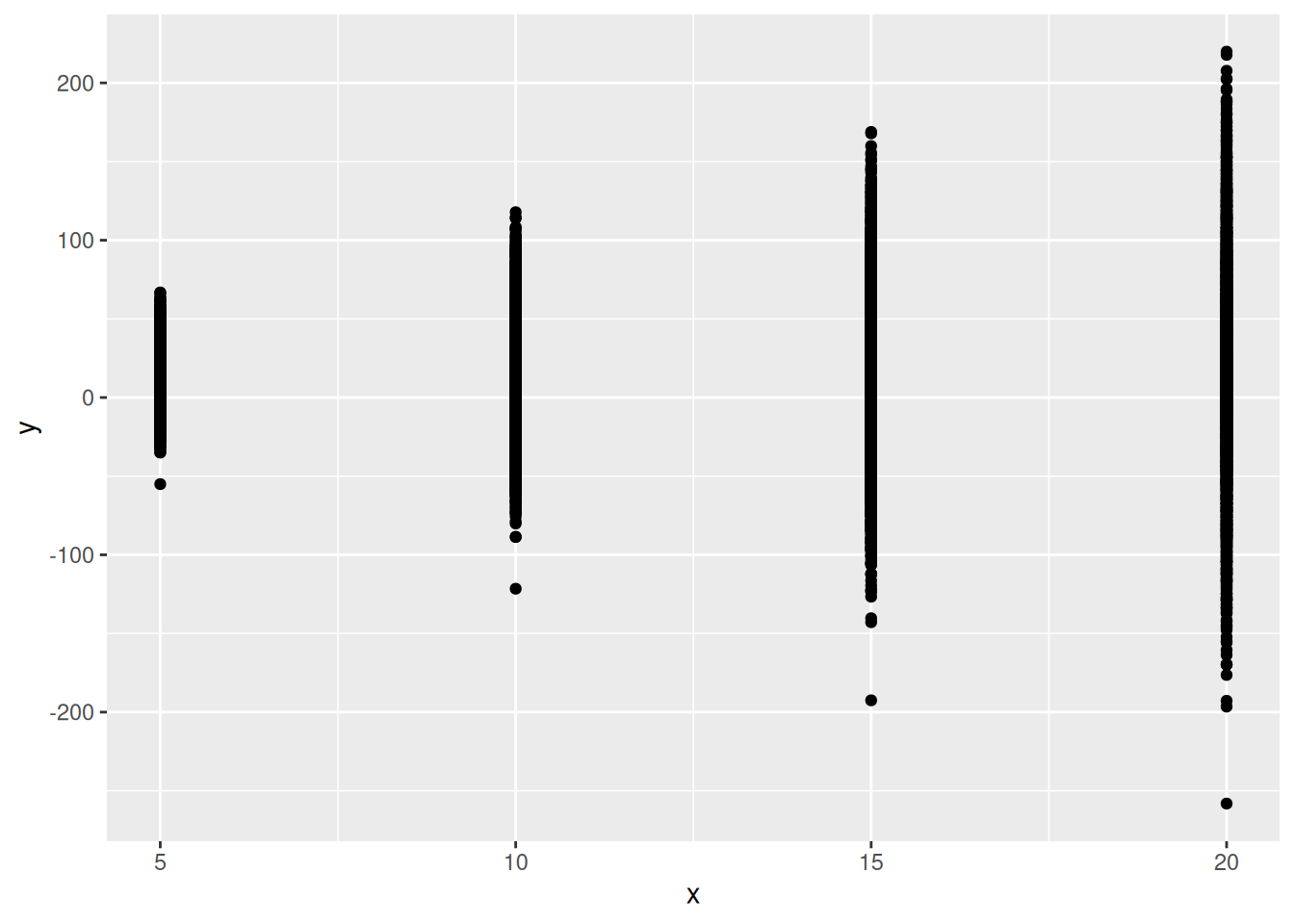
The four values of y, in the columns y[1] through y[4], are the simulated values of y that go with our four values of x. It would be nice to plot the values of y against the values of x they go with, but that requires a bit of reorganization first:¹

draws %>% 
  select(starts_with("y")) %>% 
  pivot_longer(everything(), names_to = "which", values_to = "y") %>% 
  mutate(index = parse_number(which)) %>% 
  left_join(enframe(x), join_by(index == name)) %>% 
  rename(x = value) %>% 
  ggplot(aes(x = x, y = y)) + geom_point()

Warning: Dropping 'draws_df' class as required metadata was removed.

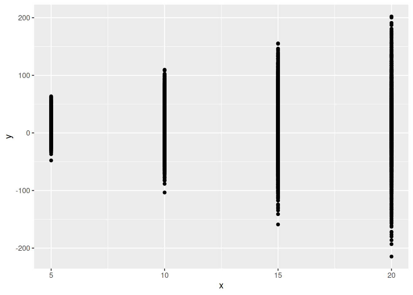
Let’s suppose that we are expecting the values of y to be positive, and so the values we got here are too variable, especially for larger values of x. The thing that controls the variability, as we have set it up, is the value of theta (the prior mean of the exponential distribution for sigma is 1/theta). So, to make the values of y less variable, we need to make theta bigger. Let’s try making it ten times bigger. Reset and repeat:

sim <- reg_prior$sample(data = list(n = 4, x = x, theta = 10))
draws <- sim$draws(format = "df")
draws %>% 
  select(starts_with("y")) %>% 
  pivot_longer(everything(), names_to = "which", values_to = "y") %>% 
  mutate(index = parse_number(which)) %>% 
  left_join(enframe(x), join_by(index == name)) %>% 
  rename(x = value) %>% 
  ggplot(aes(x = x, y = y)) + geom_point() -> g

Footnotes

Which I am not going to explain.↩︎