── Attaching core tidyverse packages ──────────────────────── tidyverse 2.0.0 ──
✔ dplyr     1.2.1     ✔ readr     2.2.0
✔ forcats   1.0.1     ✔ stringr   1.6.0
✔ ggplot2   4.0.3     ✔ tibble    3.3.1
✔ lubridate 1.9.5     ✔ tidyr     1.3.2
✔ purrr     1.2.2
── Conflicts ────────────────────────────────────────── tidyverse_conflicts() ──
✖ dplyr::filter() masks stats::filter()
✖ dplyr::lag()    masks stats::lag()
ℹ Use the conflicted package (<http://conflicted.r-lib.org/>) to force all conflicts to become errors
library(cmdstanr)
This is cmdstanr version 0.9.0.9000
- CmdStanR documentation and vignettes: mc-stan.org/cmdstanr
- CmdStan path: /home/ken/.cmdstan/cmdstan-2.39.0
- CmdStan version: 2.39.0
Introduction
A Bayesian statistician needs not only a model for the data-generation process, but also a prior distribution, which captures their beliefs or knowledge about what they would expect without looking at the actual data. Some people advocate priors that reflect ignorance about the parameters being estimated, but this comes with additional baggage (that we will see later). It is more appropriate to use a “weakly informative” prior that captures a belief that certain kinds of observations are reasonable and others are not.
But, how to specify such a prior? One way is to choose a family of prior distributions, and then choose the parameters to match the mean and variance, or percentiles, based on what you would expect to see. Another way is to obtain simulated data from the prior predictive distribution based on a choice of prior, and to decide whether that looks like the kind of data you would expect. If not, adjust the prior and try again.
As well as enabling us to sample from a posterior distribution, Stan also enables us to sample from a prior distribution, and the purpose of this blog post is to demonstrate how this can be done.
We take a (deliberately) simple example, to illustrate the procedure.
Example: estimating a Poisson mean
Let’s suppose we are going to collect data that we believe will be independent and identically Poisson distributed, with a mean that we want to estimate. We believe that a prior gamma distribution for the mean is reasonable (on the basis that the mean must be positive but is otherwise unrestricted), but we don’t know what parameters it should have yet. In Stan, a gamma distribution has two parameters alpha and beta, with the ratio of them being the mean.
I’m going to start by writing the actual Stan program that will be used later to do the estimation. Here’s mine, saved in poisson.stan:
data {
  int<lower=0> n;
  array[n] int y;
  real<lower=0> alpha;
  real<lower=0> beta;
}

parameters {
  real<lower=0> lambda;
}

model {
  lambda ~ gamma(alpha, beta);
  y ~ poisson(lambda);
}
The way I write these is to start with the data-generation process: my data values y each have a Poisson distribution with mean lambda. lambda is a parameter so it needs a prior distribution: gamma with thus-far unknown parameters alpha and beta. These two lines complete the model section.
The parameters and data sections above are then housekeeping. There is only one parameter, lambda (which is a positive real number). Everything else will be fed in as data: y is an array of integer observations, of a certain length n that we will also need to input, along with the parameters alpha and beta of the prior distribution, also positive real numbers.
At this point, it is probably smart to check that this compiles:
The observations have mean 2, and the prior mean is 1, so a posterior mean like this is entirely reasonable.
Prior predictive distribution
The point of this exercise is to choose values for alpha and betawithout having any data, just our prior beliefs or knowledge. Stan will let you sample from your prior distribution and simulate the kind of observations that will come from it; then you can eyeball these simulated observations and see whether they are in line with what you would expect. To do that, we start by taking our Stan code and removing any reference to any actual data, as well as the parameters section:
data {
  real<lower=0> alpha;
  real<lower=0> beta;
}

model {
  lambda ~ gamma(alpha, beta);
  y ~ poisson(lambda);
}
Now we have to replace the model section by a generated quantities section that conveys the same intent: lambda is a random value from the gamma distribution shown, and, given that, y is a random Poisson value whose mean is that value of lambda. Stan has functions for each of its distributions that are random number generators with _rng on the end of their names, giving this:
data {
  real<lower=0> alpha;
  real<lower=0> beta;
}

generated quantities {
  real lambda = gamma_rng(alpha, beta);
  int y = poisson_rng(lambda);
}
Note that now, lambda and y have not been previously declared, so we have to declare them as real and int. In this code, alpha and beta are “data”, in the sense that we are going to want to simulate data from prior distributions with several different values of these parameters.
This is, despite appearances, a complete Stan program, so we can compile it too:
Now, we want to sample from this. Our prior knowledge is (let’s suppose) that the observations we will observe should be about 2 on average, and that any observed values bigger than about 10 should be rare. We might happen to have heard that a not-too-informative prior has small values for alpha and beta, so, to get the average right, let’s try 0.2 and 0.1:
 variable mean median   sd  mad   q5   q95 rhat ess_bulk ess_tail
   lp__   0.00   0.00 0.00 0.00 0.00  0.00   NA       NA       NA
   lambda 1.98   0.20 4.53 0.29 0.00 10.17 1.00     3844     3929
   y      1.99   0.00 4.80 0.00 0.00 11.00 1.00     3995     3977
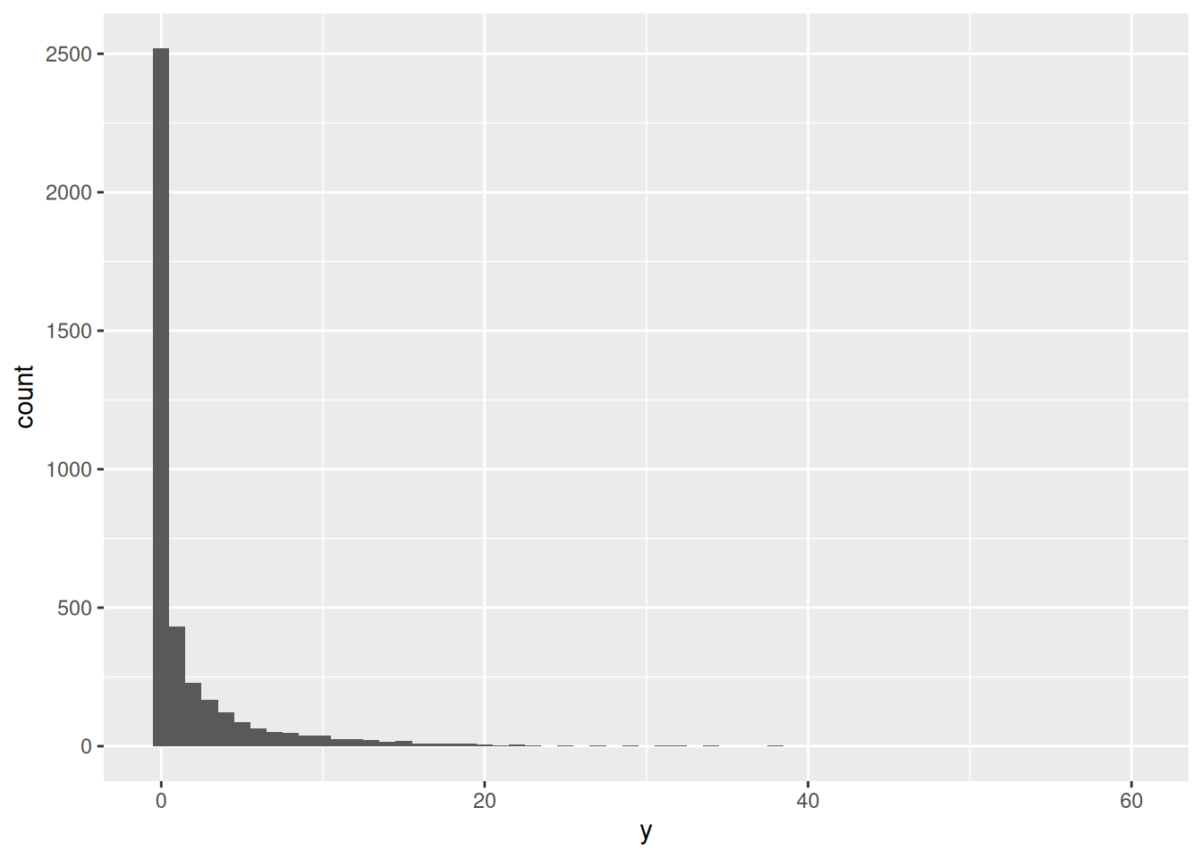
The values in y are our simulated prior predictive distribution. They have about the right mean, but it looks (from the 95th percentile) as if they go up a bit too far. To verify this, we can obtain the actual simulated values:
draws <- poisson_prior_sample$draws(format ="df")draws
at which point it becomes clear that they go up way too high: there is a non-trivial chance of obtaining observations above 20 if we use this prior distribution, and therefore this prior does not reflect our actual prior knowledge.
This prior is too weakly informative: we know more about the likely observations than this. Here, we see the problem with using a prior that is not informative enough: it says that values we know to be unlikely or impossible are in fact possible or likely under that prior, and it does not reflect our prior knowledge.
We should, perhaps, have seen this coming. The variance of a gamma distribution parameterized as Stan does it is alpha divided by beta squared, and so the standard deviation is
sqrt(0.2/0.1^2)
[1] 4.472136
which suggests that the distribution will contain too many large values. It is easier to see, though, by actually simulating the prior predictive distribution and seeing what kind of values it contains: looking at the SD forces us to make a guess about what will happen.
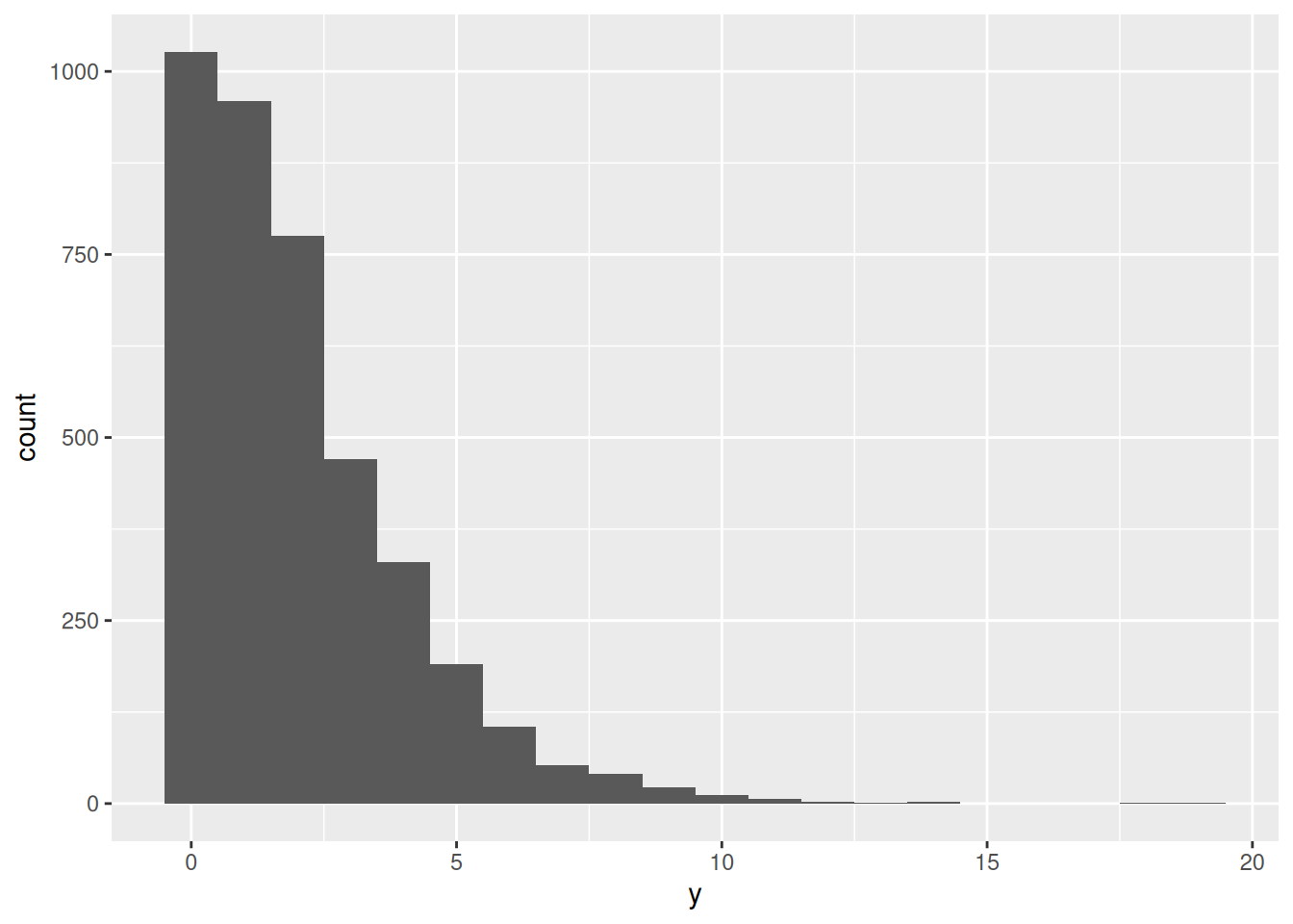
With all this in mind, maybe some values like 2 and 1 will be better:
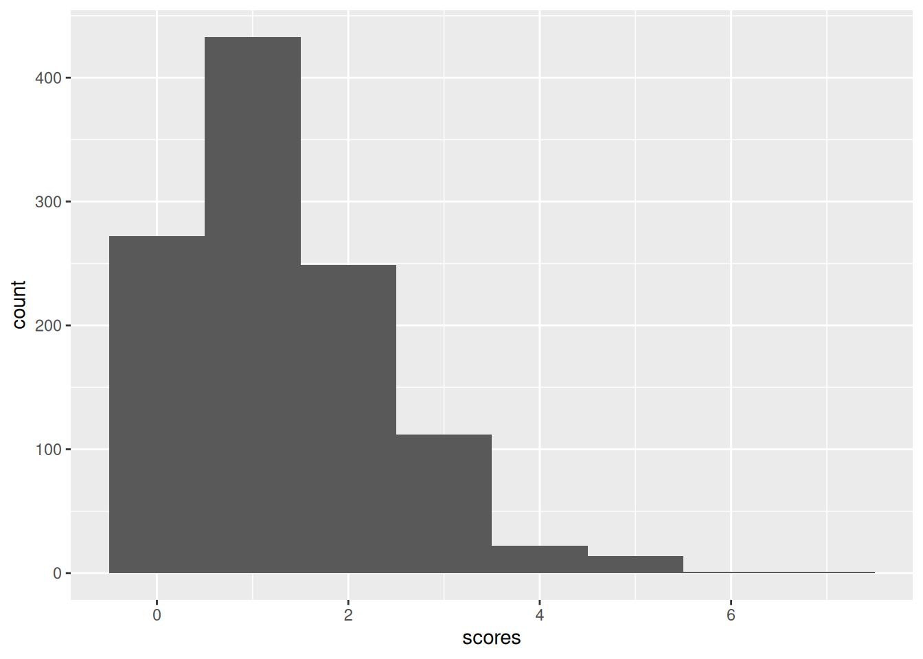
I happen to have the scores from all the games in the 2025-2026 English (soccer) Championship. Under the undoubtedly unreasonable assumption that each number of goals scored by each team in each game is independently Poisson with the same mean, we can estimate what that same mean is.
Here are the first few scores:
scores[1:20]
[1] 1 1 0 2 1 1 0 1 3 1 1 2 3 1 2 1 0 0 2 0
There are 1104 scores altogether, saved in a vector scores, so using the prior we just developed, we get
With so much data, we obtain a very tight posterior 90% interval for the mean, and in contrast to our prior knowledge, the mean is actually less than 2. It undoubtedly didn’t matter much, in the end, what prior distribution we used, but we can rest assured that the prior distribution we did use actually did reflect our prior beliefs.
Posterior predictive distribution
In the same way as we obtained the prior predictive distribution, we can obtain the posterior predictive distribution: that is, the posterior distribution of goals scored incorporating both our prior beliefs and the data. This helps us answer a question like “how likely is it that a team scores 5 or more goals” on the basis of our model. In addition, we can compare the posterior predictive distribution with the distribution of our data; if these disagree too much, it indicates a problem with our model.
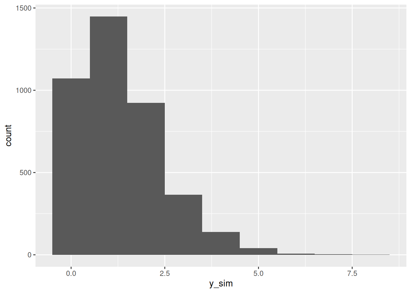
To obtain the posterior predictive distribution, we use a generated quantities section as we did when obtaining the prior predictive distribution. This time, we add it to our Stan code, and since we already used the name y in our model, we use a different name:
generated quantities {
  int y_sim = poisson_rng(lambda);
}
This says “for each value of lambda in the sampled posterior distribution, generate a random Poisson value with that value of lambda”.
They look not very different in shape, and so the model seems to be about right.
Looking ahead
This was, of course, a very simple model. In most cases, the model will have more of a regression or ANOVA flavour, with a response variable and one or more explanatory variables. Each combination of explanatory-variable values will have its own prior predictive distribution of values for the response, and in principle all of those will need to be checked for reasonableness.
In practice, it may be reasonable to simplify things, such as to restrict the search for prior distributions for a slope to those that have mean zero. The section on posterior and prior predictive checks in the Stan documentation shows what can be done.