How far apart are two clusters of objects, when all I have are distances between objects?
Hierarchical cluster analysis is based on distances between individuals. This can be defined via Euclidean distance, Manhattan distance, a matching coefficient, etc. I won’t get into these further.
There is a second problem, though, which I do wish to discuss: when you carry out a hierarchical cluster analysis, you want to join the two closest clusters together at each step. But how do you work out how far apart two clusters are, when all you have are distances between individuals? Here, I give some examples, and, perhaps more interesting, some visuals with the code that makes them.
Inter-cluster distances
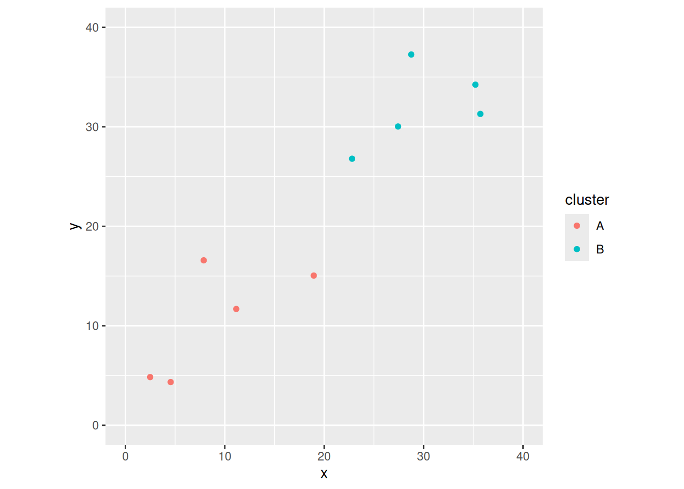
Some clusters to find differences between
Let’s make some random points in two dimensions that are in two clusters: 5 points each, uniformly distributed on \((0,20)^2\) and \((20,40)^2\):
Note that I gave this graph a name, so that I can add things to it later.
We know how to measure distances between individuals, but what about distances between clusters?
Single linkage
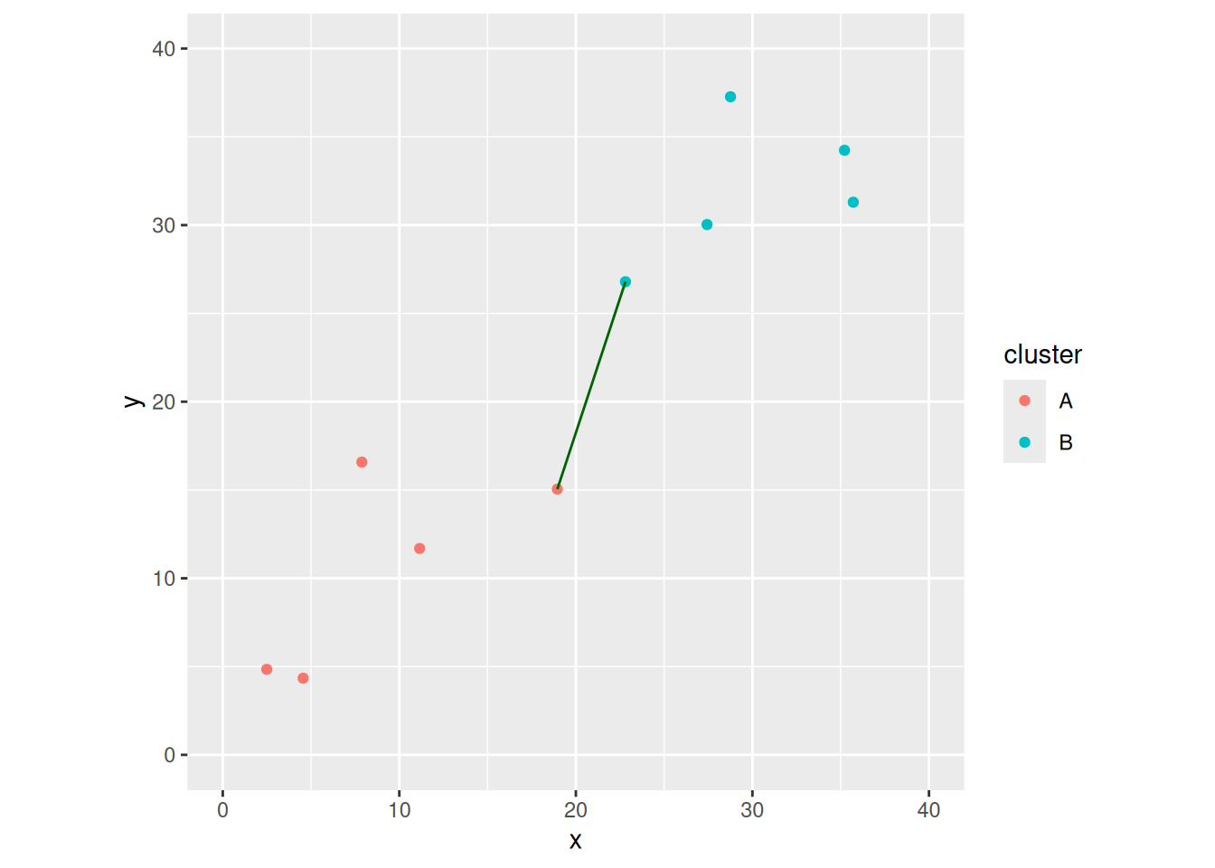
One way to measure the distance between two clusters is to pick a point from each cluster to represent that cluster, and use the distance between those. For example, we might find the points in cluster A and and in cluster B that are closest together, and say that the distance between the two clusters is the distance between those two points.
So, we need all the distances between a point in A and a point in B. The package spatstat.geom has a function crossdist that does exactly this:
This is a matrix. From this, we want to find out which points are the two that have the smallest distance between them. It looks like point 1 in A and point 3 in B (the middle distance of the top row). We can use base R to verify this:
Warning in geom_segment(data = closest, aes(x = x[1], y = y[1], xend = x[2], : All aesthetics have length 1, but the data has 2 rows.
ℹ Please consider using `annotate()` or provide this layer with data containing
  a single row.
This works, but it isn’t very elegant (or very tidyverse).
I usually use crossing for this kind of thing, but the points in A and B have both an x and a y coordinate. I use a hack: unite to combine them together into one thing, then separate after making all possible pairs:
The reason for the sep in the separate is that separate also counts the decimal points as separators, which I want to exclude; the only separators should be the underscores that unite introduced. The convert turns the coordinates back into numbers.
Now I find the (Euclidean) distances and then the smallest one:
A problem with single linkage is that two clusters are close if a point in A and a point in B happen to be close. The other red and blue points on the graph could be anywhere. You could say that this goes against two clusters being “close”. The impact in cluster analysis is that you get “stringy” clusters where single points are added on to clusters one at a time. Can we improve on that?
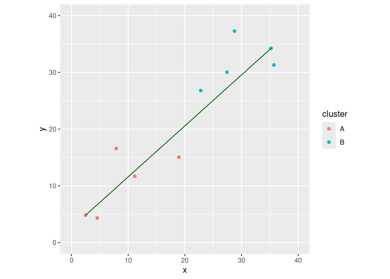
Complete linkage
Another way to measure the distance between two clusters is the longest distance between a point in A and a point in B. This will make two clusters close if everything in the two clusters is close. You could reasonably argue that this is a better idea than single linkage.
After the work we did above, this is simple to draw: take the data frame distances, find the largest distance, and add it to the plot:
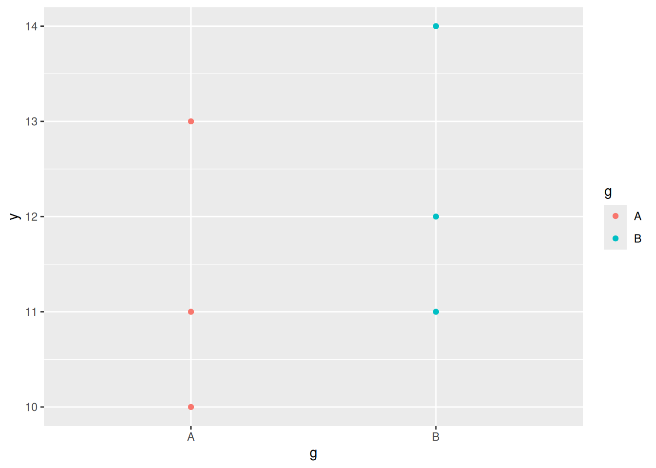
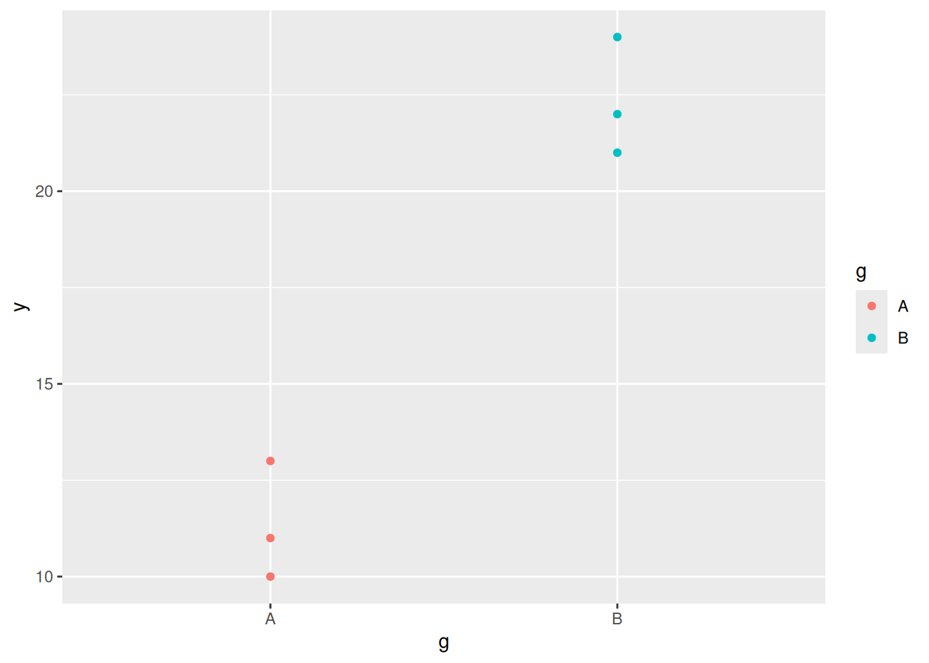
Let’s cast our minds back to analysis of variance, which gives another way of thinking about distance between groups (in one dimension). Consider these data:
# A tibble: 6 × 2
      y g
  <dbl> <chr>
1    10 A
2    11 A
3    13 A
4    11 B
5    12 B
6    14 B
The two groups here are pretty close together, relative to how spread out they are:
ggplot(d1, aes(x=g, y=y, colour=g))+geom_point()
and the analysis of variance concurs:
d1.1=aov(y~g, data=d1)summary(d1.1)
            Df Sum Sq Mean Sq F value Pr(>F)
g            1  1.500   1.500   0.643  0.468
Residuals    4  9.333   2.333
The \(F\)-value is small because the variability between groups is small compared to the variability within groups; it’s reasonable to act as if the two groups have the same mean.
# A tibble: 6 × 2
      y g
  <dbl> <chr>
1    10 A
2    11 A
3    13 A
4    21 B
5    22 B
6    24 B
ggplot(d2, aes(x=g, y=y, colour=g))+geom_point()
How do within-groups and between-groups compare this time?
d2.1=aov(y~g, data=d2)summary(d2.1)
            Df Sum Sq Mean Sq F value   Pr(>F)
g            1 181.50  181.50   77.79 0.000912 ***
Residuals    4   9.33    2.33
---
Signif. codes:  0 '***' 0.001 '**' 0.01 '*' 0.05 '.' 0.1 ' ' 1
This time the variability between groups is much larger than the variability within groups; we have (strong) evidence that the group means are different, and it makes sense to treat the groups separately.
How does that apply to cluster distances? Well, what is happening here is comparing squared distances from group means to distances from the overall mean. Let’s see:
One way to measure the distance between two groups (clusters) is to take the difference of these. The observations will always be closer to their own group mean than to the combined mean, but in this case the difference is small:
10.8-9.33
[1] 1.47
Thinking of these as clusters, these are close together and could easily be combined.
What about the two groups that look more distinct?
This is much bigger, and combining these groups would not be a good idea.
For cluster analysis, these ideas are behind Ward’s method. Compare the distances of each point from the mean of the clusters they currently belong to, with the distances from the mean of those two clusters combined. If the difference between these is small, the two clusters could be combined; if not, the two clusters should not be combined if possible.
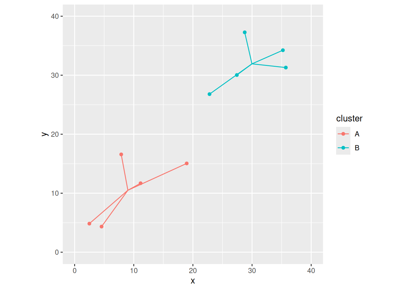
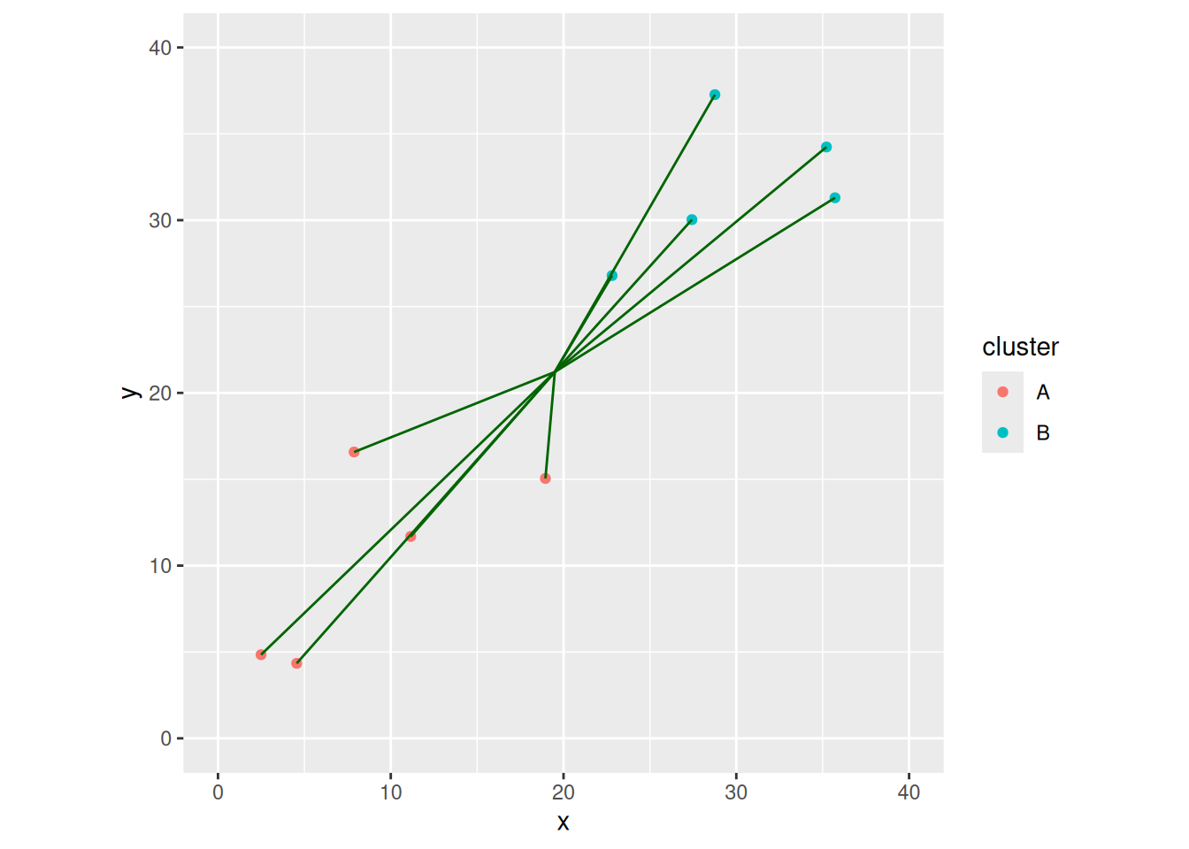
How does this look on a picture? I did this in my lecture notes with some hairy for-loops, but I think I can do better.
Let’s first work out the means for each of x and y for my clusters:
The points are a lot further from the overall mean than from the group means (the green lines overall are longer than the red and blue ones), suggesting that the clusters are, in the sense of Ward’s method, a long way apart.