How might we do a non-parametric version of two-way analysis of variance?
Introduction
In a previous post, we investigated how we might run a non-parametric version of a one-way ANOVA, for use when we are unsure about normality. I advocated for using Mood’s median test over something like Kruskal-Wallis, because the latter test comes with additional assumptions (equality of distributions apart from a difference in medians, thus implying equal spreads) that we may be uncomfortable with in practice.
There seems not to be a well-known non-parametric version of two-way ANOVA, which looks like an omission because we can face the same issues (non-normality, unequal spreads) that we face in any ANOVA analysis. Here, I propose a generalization of Mood’s median test and a way to perform the analysis.
Packages
library(tidyverse)
── Attaching core tidyverse packages ──────────────────────── tidyverse 2.0.0 ──
✔ dplyr     1.2.0.9000     ✔ readr     2.2.0
✔ forcats   1.0.1          ✔ stringr   1.6.0
✔ ggplot2   4.0.2          ✔ tibble    3.3.1
✔ lubridate 1.9.5          ✔ tidyr     1.3.2
✔ purrr     1.2.2
── Conflicts ────────────────────────────────────────── tidyverse_conflicts() ──
✖ dplyr::filter() masks stats::filter()
✖ dplyr::lag()    masks stats::lag()
ℹ Use the conflicted package (<http://conflicted.r-lib.org/>) to force all conflicts to become errors
library(isdals) # for datalibrary(Devore7) # also for data
Loading required package: MASS

Attaching package: 'MASS'

The following object is masked from 'package:dplyr':

    select

Loading required package: lattice
library(smmr) # for running a regular Mood's median test
Example 1: listeria data
We use the listeria data from the isdals package. To quote from the help file:
Ten wildtype mice and ten RIP2-deficient mice, i.e., mice without the RIP2 protein, were used in the experiment. Each mouse was infected with listeria, and after three days the bacteria growth was measured in the liver or spleen. Errors were detected for two liver measurements, so the total number of observations is 18.
The response variable is the bacteria growth, and this might depend on the organ where the measurement was taken, and the type of mouse (wildtype or RIP-deficient). The data look like this:
data(listeria)listeria
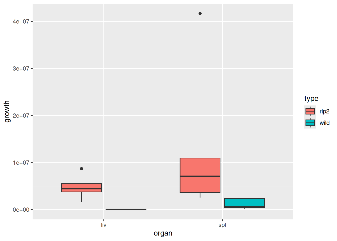
A standard graph with data of this type is a grouped boxplot, like this:
ggplot(listeria, aes(x = organ, y = growth, fill = type)) +geom_boxplot()
There are some serious problems with outliers, and even discounting that, the spreads do not look very equal. We might consider a transformation here (indeed, there might be a good scientific reason for looking at something like the log of growth), but aside from that, what can we do?
Re-purposing Mood’s median test
Recall that the idea behind Mood’s median test was to replace the response variable by a categorical version of itself,1 indicating whether it was above or below the grand median of all the data:
Now we have three categorical variables. In particular, we are looking for an association between above_below and either or both of the other (explanatory) categorical variables. Since we have more than two categorical variables, we can no longer use an ordinary chi-squared test, but in this post we saw that an appropriate analysis is a log-linear model. To do that, we need the number of observations for each combination of levels of each categorical variable, but this doesn’t quite do it:
listeria %>%count(organ, type, above_below)
The problem is that count only includes the nonzero counts, and for the analysis, we need all the combinations of categories, including the zero counts. (There should be \(2^3 = 8\) rows here.) You would think that asking count not to drop any counts would work, but:
This doesn’t work either. For the .drop option to work properly, all the categorical variables need explicitly to be factors. (The documentation sort-of implicitly says this, but doesn’t explicitly say that categorical variables need to be factor rather than text.)
listeria.3<-update(listeria.2, . ~ . - organ:type)drop1(listeria.3, test ="Chisq")
and the one remaining non-significant effect:
listeria.4<-update(listeria.3, . ~ . - organ:above_below)drop1(listeria.4, test ="Chisq")
and the non-significant main effect:
listeria.5<-update(listeria.4, . ~ . - organ)drop1(listeria.5, test ="Chisq")
and we are done, with everything significant. In the model, there is a significant interaction between mouse type and whether or not their growth was above or below the grand median; that is to say, there is a significant association between the two variables. In this case, above_below is logically the response variable, so we can say that knowing a mouse’s type tells us about their growth (or, to be more precise, tells us whether their growth is above or below the median of all growth values). We have, in other words, found a significant type main effect.
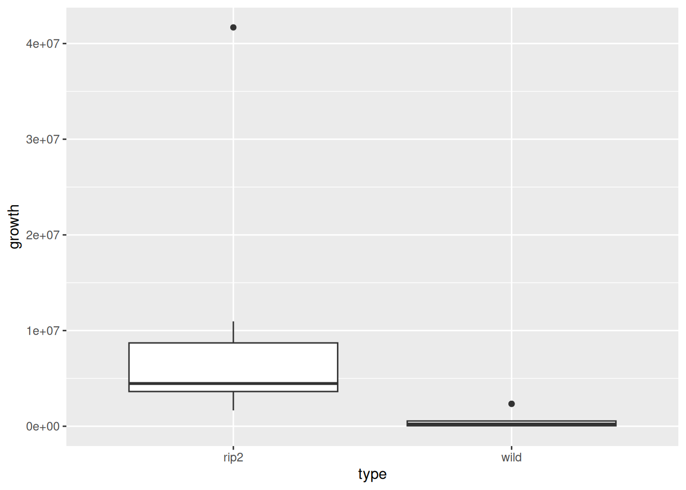
To see what kind of effect it is, the other post said to look at graphs of the categorical variables concerned, but here we have the actual growth values, so we can look at an ordinary boxplot (with the quantitative growth values and the categorical type):
ggplot(listeria, aes(x = type, y = growth)) +geom_boxplot()
This tells us that the median growth for RIP2-deficient mice is greater than for the wild-type mice, and that was the reason for the significant type effect.
On the other hand, the organ:above_below term was removed from the model, so there is no significant effect of which organ the measurement was taken from on the amount of bacteria growth. Nor is there a significant interaction effect of organ and type (because the organ:type:above_below term was removed from the model early on).
Example 2: uniformity of coating
Devore, in exercise 11.53 of Probability and Statistics for Engineering and the Sciences (7th ed), gives data for a replicated \(2^3\) factorial design described as follows:
In an automated chemical coating process, the speed with which objects on a conveyor belt are passed through a chemical spray (belt speed), the amount of chemical sprayed (spray volume), and the brand of chemical used (brand) are factors that may affect the uniformity of the coating applied. A replicated \(2^3\) experiment was conducted in an effort to increase the coating uniformity. In the following table, higher values of the response variable are associated with higher surface uniformity.
The response variable is a (quantitative) measure of surface uniformity, and the three explanatory variables (factors) are belt speed, spray volume, and brand of chemical used. The two levels of each factor are denoted “+” (high) and “-” (low). In the original data there were two replicates at each factor combination; in our analysis, we ignore brand to leave us with a \(2^2\) factorial design with four observations at each combination of belt speed and spray volume.
The data are as shown:
data(ex11.53)ex11.53
This needs a little reformatting to get all the response variable values into one column:
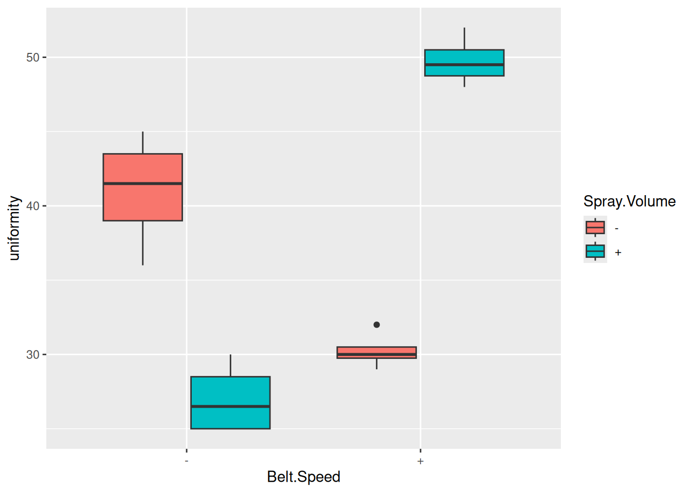
We can draw a grouped boxplot in an attempt to assess normality and equal spreads:
ggplot(ex11.53a, aes(x = Belt.Speed, fill = Spray.Volume, y = uniformity)) +geom_boxplot()
The problem with higher-order ANOVAs is that each box on a boxplot like this is typically based on very few observations (four, in this case), which makes it difficult to assess normality and equal spreads. There is an outlier here and some very vague evidence of unequal spreads (eg. a smaller spread when both factors are high, and a larger one when both factors are low), but it is virtually impossible to say whether this is indicative of anything or just chance.2
Supposing that we wish to use the Mood’s median test idea again, we work out the grand median and whether each observation is above it or below:
I got ahead of the game here: recognizing that I was going to be using count with .drop, I made sure that above_below would also be a factor when I created it. This makes sure that we get eight rows including the zero frequencies.
Note that the frequencies are very unbalanced: the observations in a factor combination are either all above the grand median or all below.
We have three categorical variables: the two original factors, plus above_below which is a proxy for uniformity. So we fit a log-linear model:
unif.1<-glm(n ~ Spray.Volume * Belt.Speed * above_below, family ="poisson", data = unif.tab)drop1(unif.1, test ="Chisq")
In this model, the three-way interaction between cannot be dropped (P-value \(2.5 \times 10^{-6}\)), so there is a significant association in the multiway table between spray volume, belt speed, and above/below. This means that the combination of spray volume and belt speed affects whether an observation has uniformity above or below the grand median: that is, there is a significant interaction between spray volume and belt speed.
It is pretty clear from the boxplot why there is a significant interaction: when belt speed is low, uniformity is higher when spray volume is also low, but when belt speed is high, uniformity is higher when spray volume is high. (The effect of spray volume depends on the level of belt speed.)
It seems unlikely that the effects seen on the boxplot are just chance, but if we want to investigate further, we can. In regular ANOVA, a standard way of investigating a significant interaction is to use “simple effects”: fix the level of one of the factors, and investigate the effect of the second factor at that level of the first one. To do that in this context, we can (for example) look only at the observations where belt speed is low and see whether there is a significant difference in uniformity between the two different spray volumes at that belt speed. This looks like a one-way ANOVA (or two-sample test), which we can do using a regular Mood’s median test:3
$grand_median
[1] 33

$table
     above
group above below
    -     4     0
    +     0     4

$test
       what       value
1 statistic 8.000000000
2        df 1.000000000
3   P-value 0.004677735
There is a significant difference in uniformity for the different spray volumes when belt speed is low. As the boxplot revealed, this is because uniformity is greater when the spray volume is low.
In the same way, we can see whether there is an effect of spray volume when belt speed is high:
$grand_median
[1] 40

$table
     above
group above below
    -     0     4
    +     4     0

$test
       what       value
1 statistic 8.000000000
2        df 1.000000000
3   P-value 0.004677735
There is also a significant difference in uniformity between different spray volumes when belt speed is high. Looking back at the boxplot, this is because uniformity is higher when the spray volume is high.
Example 2 revisited, but with brand
In Example 2, I ignored brand. Can I include it? There is nothing in this kind of analysis restricting us to two factors. The grand median has not changed, so the only modification is to add Brand to the table of counts:
and then we fit a (slightly more complex) log-linear model:
unif.2<-glm(n ~ Spray.Volume * Belt.Speed * Brand * above_below, family ="poisson", data = unif.tab)drop1(unif.2, test ="Chisq")
This time the four-way interaction is not significant, and should be removed. The model-building process in cases like these is rather long; we can use step to do the backward elimination for us:4
unif.3<-step(unif.2, trace =0)drop1(unif.3, test ="Chisq")
We end up at the same place as before. Brand has entirely disappeared from the model, indicating that it has no effect on uniformity.
Discussion
The usual criticism levelled at Mood’s median test (and its one-sample counterpart the sign test) is that it lacks power. With small samples, and the fact that it uses the response variable inefficiently, this is a valid criticism if the actual value of the response variable is meaningful. In the cases where a normal theory analysis applies, it should of course be preferred. But when there are outliers or skewed distributions within groups, it is not clear that the response variable values are meaningful on more than an ordinal scale, and even ranks can be questionable (when the distributions within groups are skewed or have unequal spreads, an observation can receive a very high or low rank because of the distribution within its group, not because its group median is different from the others).
As with the sign test and Mood’s median test applied to two samples or one-way ANOVA, a significant result is only likely to be obtained in the case of severe imbalance (as in our second example) or samples that are at least moderate in size. In the latter case, the normality may be of lesser importance, but a larger sample does not obviate the requirement in two-way and factorial ANOVA for equal spreads. This generalization of Mood’s median test is valid5 no matter what the distributional shape and whether or not the groups have equal spreads, and thus deserves consideration in practice.
Footnotes
Categorizing a quantitative variable is usually a bad idea, but the attitude we are taking here is that the actual numeric value is not something we feel able to model.↩︎
A way to go in this situation is to run the ANOVA as a regression using lm, obtain the sixteen residuals, and assess those for normality such as with a normal quantile plot. This is more likely to reveal any real problems.↩︎
This uses median_test from my smmr package. See here for installation instructions for that package.↩︎
The trace is to stop step from displaying a considerable amount of output as it works.↩︎
From a technical point of view, there may also be issues with the quality of the chi-squared approximations in the likelihood ratio tests used in the model building for the log-linear models, and with the effect of backward elimination on the P-values. These are issues that deserve to be explored. They do not affect the validity of the test, but may affect the accuracy of the P-values obtained, particularly for small samples.↩︎